Using t-SNE, as dimensionality reduction for fraud detection

Introduction to t-SNE

t-SNE was introduced by van der Maaten and Hinton in 2008, in a foundation paper published in the Journal of Machine Learning Research, as a dimensionality reduction technique :

“dimensionality reduction methods convert the high-dimensional data set X = {x1, x2,…, xn} into two or three-dimensional data Y = {y1, y2,…, yn} that can be displayed in a scatterplot”. One main benefit of t-SNE being that t-SNE is capable of capturing much of the local structure of the high-dimensional data very well, while also revealing global structure such as the presence of clusters at several scales.

Core concepts to understand t-SNE

In order to understand t-SNE, some concepts were introduced:

• Similarity. The similarity of one datapoint xj to another datapoint xi is the conditional probability pj|i, that xi would pick xj as its neighbor if neighbors were picked in proportion to their Gaussian probability density centered at xi.
• Perplexity. Perplexity is a defined as a measure for information as 2 to the power of the Shannon entropy. Perplexity is a parameter set up by the data scientist so to instruct the algorithm to measure the effective number of neighbors. van der Maaten and Hinton suggests to use perplexity values in the range [5 - 50] and to use a higher perplexity for larger datasets.

Non reproducibility of t-SNE visualizations

As t-SNE has a non-convex objective function, minimized using a gradient descent optimization initiated randomly, so different algorithm runs can give different visualizations.

How does t-SNE work?

t-Distributed Stochastic Neighbor Embedding (t-SNE) reduces dimensionality using Barnes-Hut approximations. It maps high dimensional data to two or more dimensions, suitable in order to visualize their relationships using a stepped approach:

1. Computation of pairwise affinities pj|i in the high dimensional space by conversion of the high-dimensional Euclidean distances between data points into high dimension conditional probabilities pj|i that represent similarities, and constrained by the user defined perplexity Perp. In the high-dimensional space, the conversion of distances into probabilities is done using a Gaussian distribution.
2. Computation of a pairwise affinities in the low dimension space, as conditional probability qj|i for the low-dimensional counterparts yi and yj of the high-dimensional datapoints xi and xj, so to model pairwise similarities. In the lower-dimensional map, a Student t-distribution with one degree of freedom is used to convert distances into probabilities (so to avoid the “crowding problem”)

To Create the low-dimensional data representation, t-SNE reduces the mismatch between the corresponding high and low dimension conditional probabilities by minimizing the sum of Kullback-Leibler divergences over all datapoints using a gradient descent method whose cost function is designed so to retain the nearby map points, favoring the local structure of the data in the map.

Unlike SNE, t-SNE uses a symmetrized version of the SNE cost function with simpler gradients and a Student-t distribution rather than a Gaussian to compute the similarity between two points in the low-dimensional space.

t-SNE performed on the credit card fraud dataset

The extensive Exploratory Data Analysis of the credit card fraud dataset has been presented in this article. Here, t-SNE is a complement of the previous PCA performed on variables as the PCA, being a linear dimension reduction techniques, is not able to interpret complex polynomial relationship between features.

Data preparation for t-SNE

t-SNE is performed on the training dataset after a 70/30 partition to generate a test dataset hold out. Then the training dataset is scaled. The rescaling is necessary to have the different dimensions to be treated with equal importance.

Hyper-parameters setting for t-SNE

In this t-SNE computed with r, the tsne: T-Distributed Stochastic Neighbor Embedding for R is used. The main hyper-parameters are:

• k - the dimension of the resulting embedding
• initial_dims - The number of dimensions to use in reduction method.
• perplexity - Perplexity parameter. (optimal number of neighbors)
• max_iter - Maximum number of iterations to perform.

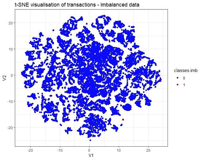
Using t-SNE visualization on an imbalanced dataset

From the training dataset of instances, I have randomly sampled the observations so to get a subset of the initial unbalanced dataset. As shown in the figure below, t-SNE is able to separate legitimate and fraudulent transactions despite the minority instances for the fraudulent transactions.

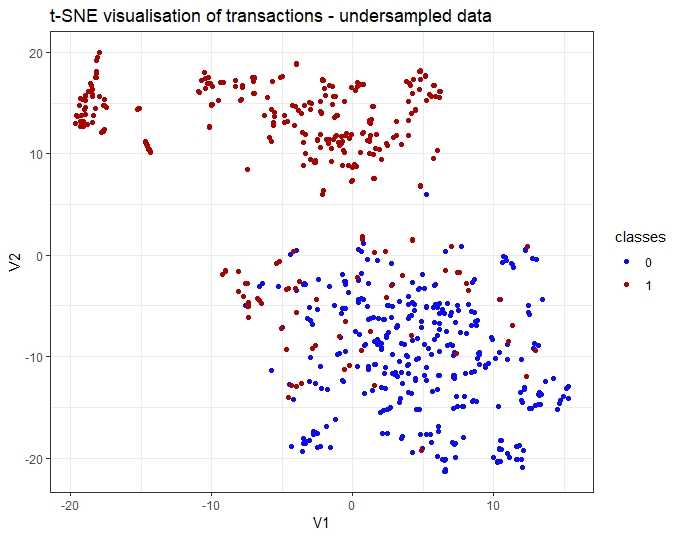
Using t-SNE visualization on a balanced dataset

The dataset was balanced by using r ROSE OVUN module so to reach an even distribution of fraud and legitimate transactions. The resulting t-SNE spots efficiently the binary classification of the target Class.

Conclusion of the t-SNE

t-SNE provides a robust way of distinction between fraudulent and legitimate transactions. In addition, the comparison between the two visualizations has shown the interest of dataset re-sampling techniques as an initial step prior to any modeling so to improve discrimination at the learning stage. Comparing those sampling / balancing techniques are the main topic of a further article. In the rest of this project, no further dimensionality reduction technique will be used so to model with all the features provided. For further reference on t-SNE, and additional examples, in other field of activity than the banking industry or the fraud prevention, the tsne official website is a starting point