Techniques to handle imbalanced dataset

Data science to prevent financial fraud

The role of the data scientist in financial fraud prevention

In financial fraud prevention, here credit card fraud, the aim of the data scientist is to develop a scalable classification model so the company can accurately classify transactions as either legitimate or fraudulent. To do so, the data scientist uses a pre-labelled dataset, comprising fraudulent and legitimate transactions, so to train, validate and test its models.

Dealing with imbalanced financial fraud data

Fraudulent transactions are the target class to be detected by the model but it is also the minority class, far outnumbered by the legitimate transactions class. An in depth exploratory data analysis, of the dataset used for this project, is provided in a previous article showing the imbalance and other variables characteristics. The target class (frauds) accounts for 0.172% of all transactions

Classification on imbalanced data

Challenges of assessing classifier performance

The following usual metrics or visualizations are proven not to be significant for performance assessment of classification models on imbalanced dataset:

Accuracy = (TP+TN) / (TP+FN+FP+TP)

• Accuracy. As the model goal is to achieve a high rate of correct detection in the minority class, allowing a small error rate in the majority class, Accuracy is not appropriate in the case of fraud detection. Kappa. Kappa or Cohen’s Kappa is a normalized measure of Accuracy.

ROC curve is a 2d plot:

• the X-axis represents FPR = FP/(TN + FP) = 1 - Specificity where Specificity = TN / (TN + FP))
• the Y-axis represents TPR = TP/(TP + FN) aka Recall

• ROC curve. ROC (Receiver Operating Characteristics) curve displays the TPR (True Positive Rate also called Recall) against the FPR (False Positive Rate) through various probability thresholds. The ROC curve gives insights on the model ability to distinguish between the classes so it is most suitable when, as data scientist, we want to design a model that predicts equally both positive and negative classes.

Metrics - Precision

Precision = TP/(TP+FP)

Precision measures the probability of a sample classified as positive to actually be positive. In financial fraud, the fraud is classified as the positive class and the model is designed so to detect correctly positive samples, therefore Precision is one of the suitable metrics.

Metrics - Recall

Recall = TPR = TP/(TP+FN)

TPR (True Positive Rate also called Recall or Sensitivity) measures the actual positive observations which are predicted correctly.

Metrics - F1 score

F1 = 2 * (precision * recall) / (precision + recall)

F1 score is a compounded metrics (from Precision and Recall) measuring the effectiveness of classification. The F1-measure, the harmonic mean of precision and recall and so is a good indicator of the performance of our model as a higher F1 will help us choosing between two models.

Metrics - AUROC

Area Under the Receiver-Operating Characteristic (AUROC) is equal to the probability that a classifier will rank a randomly chosen positive instance higher than a randomly chosen negative one (assuming ‘positive’ ranks higher than ‘negative’).

Metrics - AUPRC

The Area Under the Precision-Recall Curve (AUPRC) is computed by plotting the Precision against Recall and measuring the area under this curve.

Metrics - Matthews correlation coefficients

MCC = (TP x TN - FP x FN) / sqrt( (TP + FP) x (TP + FN) x (TN + FP) x (TN + FN))

The MCC metric has been first introduced by B.W. Matthews to assess the performance of protein secondary structure prediction. Matthews Correlation Coefficient (MCC) is defined in terms of True Positive (TP), True Negative (TN), False Positive (FP) and False Negative (FN).

Visualization - Confusion matrix

The confusion matrix is described in the table below:

		Actual	class
		Actual Positive	Actual Negative
Predicted	Predicted Positive	True Positive	False Positive (Type I error)
class	Predicted Negative	False Negative (Type II error)	True Negative

The interpretation of the confusion matrix is done as follow for a binary classification problem. Reviewing the models results to effectively predict if one transaction was positive (fraud) or negative (legitimate), the confusion matrix summarizes the results:

• True Positive (TP) – When a transaction is fraudulent and is classified correctly as fraudulent.
• False Positive (FP) – When a transaction is legitimate and was predicted and classified incorrectly as fraudulent.
• True Negative (TN) – When a transaction is legitimate and is classified correctly as legitimate.
• False Negative (FN) – When a transaction is fraudulent but was classified incorrectly as legitimate.

Visualization - Precision-Recall curve

Precision-Recall curve is a 2d plot:

• the X-axis represents Recall = TPR = TP/(TP + FN)
• the Y-axis represents the Precision = TP / (TP + FP)

The Precision-Recall Curve (AUPRC) displays the relationship between

• the true positive rate (TPR) = Recall = Sensitivity
• and the Precision = TP / (TP + FP)

Data preparation approaches to deal with imbalanced data

Oversampling

Oversampling randomly replicates a number of observations from the minority class so to match the user-defined number of observations in the majority class. This replication may lead to overfitting from the duplicated minority class data then presents in the resulting training dataset.

Under sampling

Under sampling reduces the number of observations in the majority class (non-fraudulent transactions) to match the number of observations in the minority class (fraudulent transactions). Under sampling is done by randomly selecting observations from the predominant class so to matches the n observations of the minority class initially present in the dataset. Under sampling means information loss as only a portion of the data are kept to match the minority class so this technique may lead to classification models underperformance.

Both sampling

In this two-ways sampling method, the majority class is under sampled while the minority class is oversampled, at the same time, so to obtain a user defined even number of observations from each class.

Synthetic data generation - ROSE

ROSE (Random Over-Sampling Examples) aids the task of binary classification in the presence of rare classes. It produces a synthetic, possibly balanced, sample of data simulated according to a smoothed-bootstrap approach.

Synthetic data generation - SMOTE

SMOTE over-samples the minority fraudulent class by generating synthetic fraudulent data in the neighborhood of observed ones, interpolating to create those synthetic data between real observation of the same minority class. SMOTE first finds the k-nearest-neighbors for minority class observations and then randomly choose one of the k-nearest-neighbors to create this synthetic data belonging to the minority Class. One of the downsize of SMOTE is noise generation from interpolation between outliers and inliers.

Cost Sensitive Learning (CSL)

Total Cost = C(FN)xFN + C(FP)xFP where C(FN) and C(FP) are the costs associated with False Negative and False Positive respectively (C(FN) > C(FP))

This approach is a cost-based approach where the model parameters are set-up such as misclassification of the minority class is weighted differently so a high misclassification cost is attributed when predicting False Positives or False Negatives instead of, usually, weighting them equally.

Modeling - Supervised learning - Random Forest

Using a Random Forest classifier

Our model uses a Random Forest classifier in order to predict fraudulent transactions. The module used is r, RandomForest. Random Forest is an Ensemble classifier which uses first multiple decision trees as weak learners to, then, bootstrap aggregate, a process called “bagging”, the tree learners. Random Forest output is a stronger classifier.

Modeling with the Random Forest classifier

To build and develop this model, I have followed the steps:

1. Train/Test split with a 70/30 ratio
2. Separate scaling (to avoid leaking information of each subsequent dataset)
3. Hold out of the test dataset
4. Creation of 5 different datasets from the training dataset: training, training under sampled, training oversampled, training both sampled, training post-ROSE, training post ROSE.
5. Application of the Random Forest classifier on each 6 datasets (original + the 5 created by the resampling)
6. Prediction of the class on the test dataset

Random Forest on Imbalanced data

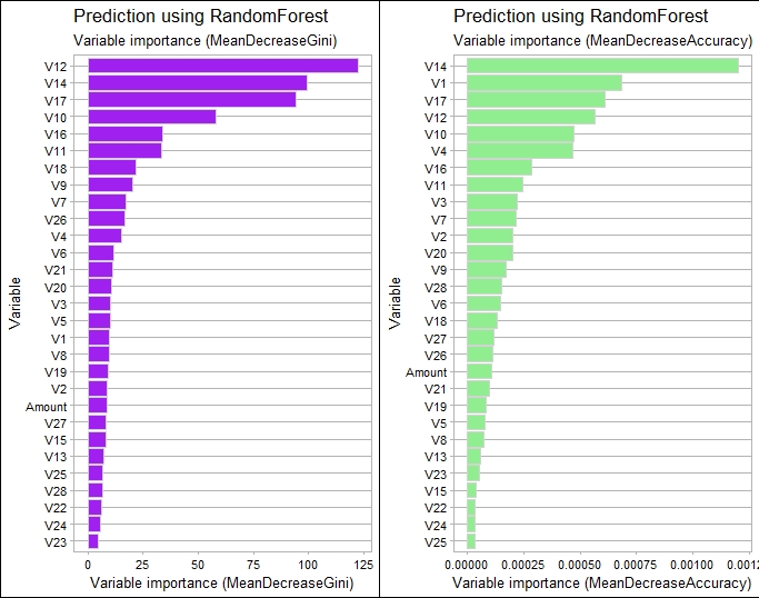
Variables importance

Following the model building, we visualize the variables importance and variables V12, V14, V17, V10 stands out as main predictors.

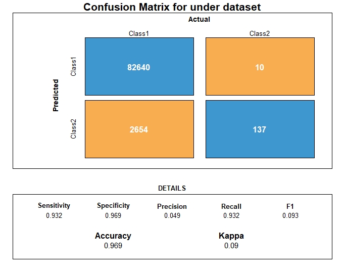
Confusion matrix

After prediction, we can then compute the confusion matrix

Random Forest on resampled data

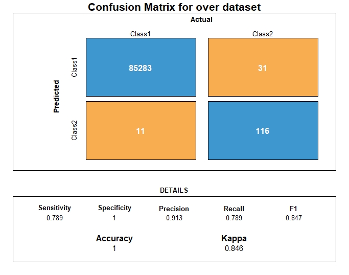
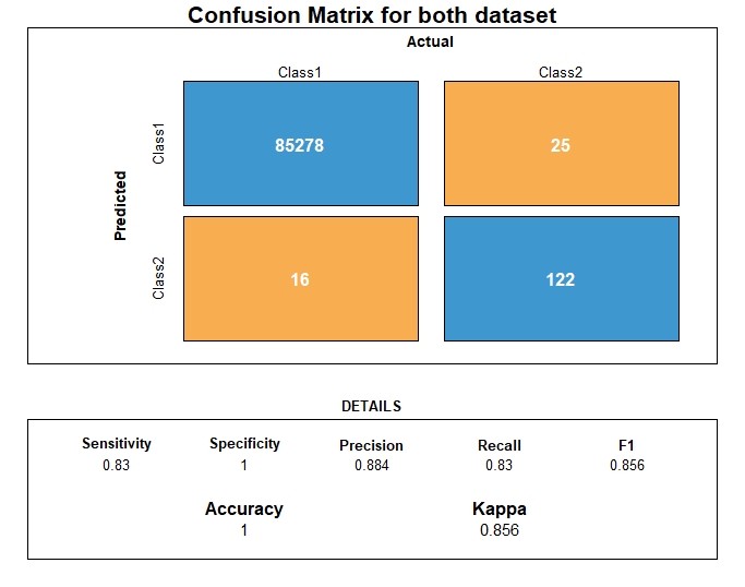
Confusion matrices

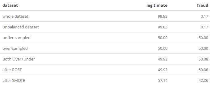
Dataset class ratio

Five training datasets were created so to be compared once the same classifier was applied. The 5 datasets were balanced.

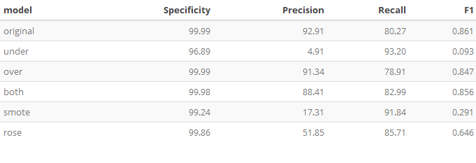
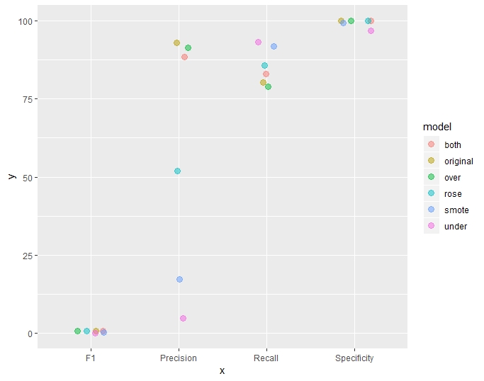
Metrics comparison

In the table and plot below, the following metrics were grouped and then plotted. SMOTE and Undersampling offers the highest Recall.

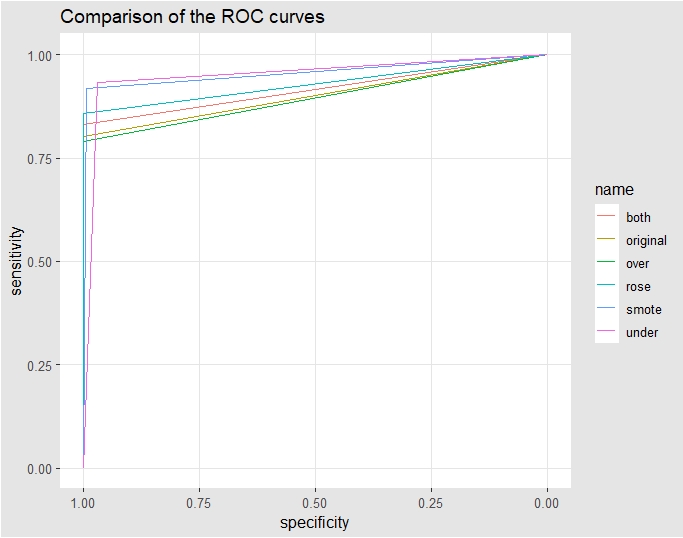
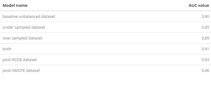
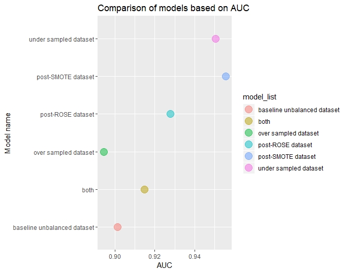
AUC comparison

Comparing the different re-sampling techniques based on AUC, AUC is higher in decreasing order for

1. SMOTE
2. Undersampling
3. ROSE

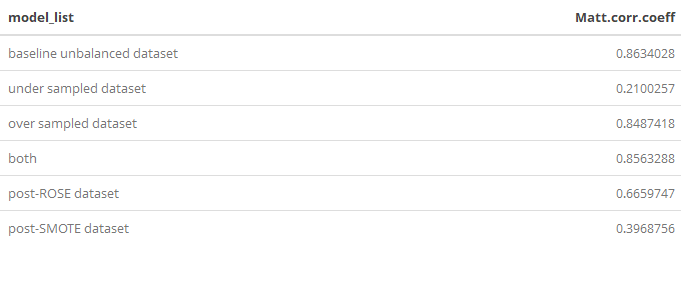
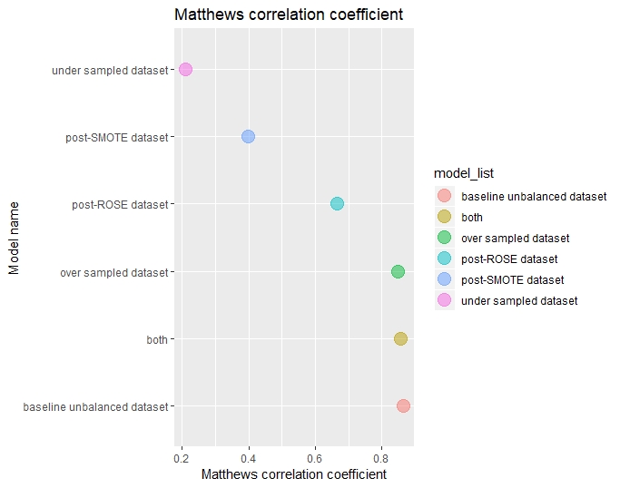
Matthews correlation coefficient comparison

For each model, the Matthews correlation coefficient were computed and compared.

Conclusion

Regarding re-sampling the training dataset, SMOTE and BOTH offers the best results. Next, a subsequent article will focus how to improve those results using other classifiers than Random Forest so to create a scalable final model.