Comparing ensemble approaches to improve model performance

Our goal is to reduce the costs of undetected fraud cases by pre-screening potential frauds. To do so, the strategy chosen is to develop a machine fraud detection model, efficient enough so to be implemented in production and ensure fraud tagging and prevention. To support this strategy, the main objective is to design and compare various machine learning algorithms and to select the most relevant as per evaluation.

Data science for fraud prevention

Designing a fraud detection machine learning solutions can be challenging because of:

1. the non-stationarity of credit card data
2. the fraudulent/legit class is imbalanced
3. the potential lack of accuracy of labelled data by fraud investigator
4. the scarcely availability of test datasets for confidentiality issues

The aim of this project is to develop a data science solutions detecting fraudulent transactions at a low latency. To do so, we will explore and compare machine learning prediction models.

What is the role of the data scientist in fraud prevention?

Within the fraud prevention team, the role of the data scientist is to use a scientific approach so to design, fine-tune, validate and test various classification algorithm models to narrow the choice with its colleagues and stakeholders to a model efficient enough to be upscaled in production.

Exploratory data Analysis

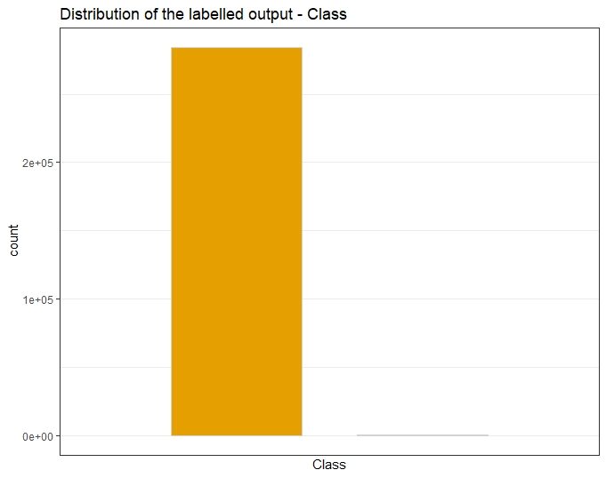
A previous in-depth Exploratory Data Analysis has analyzed the imbalance nature of this dataset with 492 fraudulent transactions out of 284,807 total transactions.

The target Class

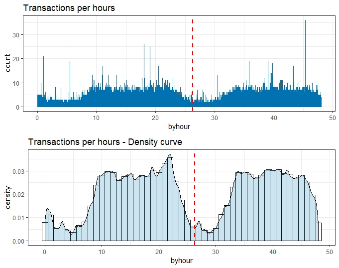
The timelime with Time

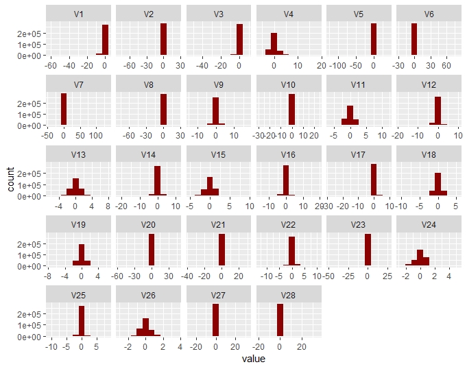
The PCA Vi Variables

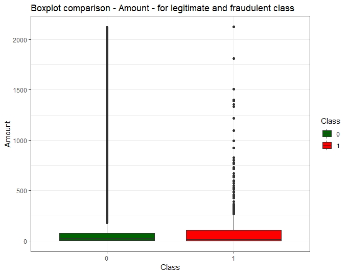
The cost dimension of fraud

Data preparation

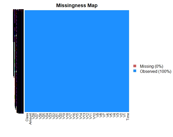
Missing data

This dataset has no missing data as plotted below.

Outlier analysis and removal

An outlier analysis has been performed including its impact on the available fraud cases. Due to the explanatory potential of some variables (V14, V12, V10) outliers, and their prevalence in the fraud Class, and so to the risk of suppressing important learning cases, if outliers removal were to be applied, the choice has been made not to apply any outliers removal technique.

Other data transformation

Scaling of variables

We can observe that due to the PCA being performed, the Vi variables are centered. As the Amount features was no scaled unlike the Vi (due to the PCA), we normalize it. To avoid “leaking” information between training and test datasets, this step is performed separately on each datasets.

Resampling of the training/validation dataset

After the train/test split so to keep the test hold-out intact, the training dataset was resampled using a both approach.

Features engineering

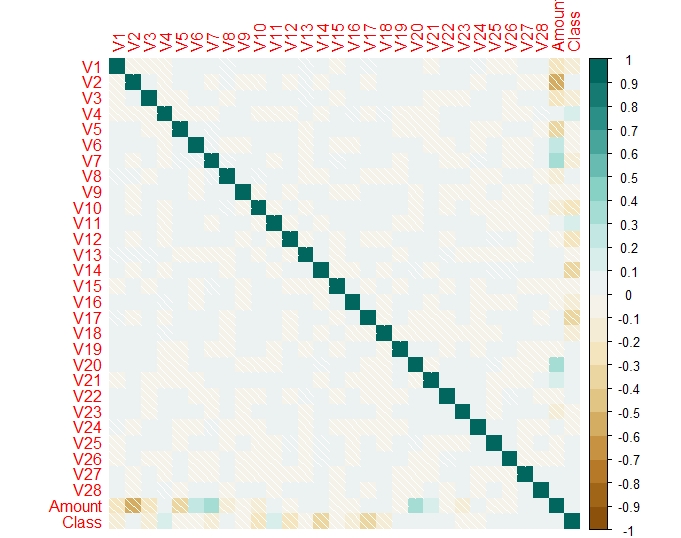
Correlation between variables

As the main Vi variables are the results of a PCA, we do no expect them to be correlated and so we check if this assumption is confirmed and I have generated the Pearson correlation for the data.

PCA

A Principal Component Analysis (PCA) has already been performed whose output are the Vi variables provided.

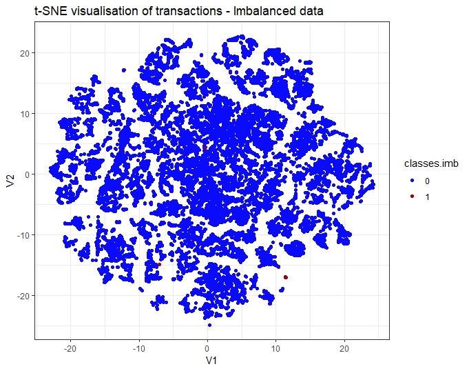
t-SNE

t-Distributed Stochastic Neighbor Embedding (t-SNE) is a non-linear technique to reduce dimensionality using Barnes-Hut approximations and I have written in a separate article about t-SNE and how it was applied to this dataset.

Model execution and evaluation strategy

Supervised learning classification

The aim of machine learning classification is to predict a discrete class label output given a data observation (characterized by multiple input variables). In supervised learning classification,

• the training dataset is supplied with the labelled output
• then, the algorithm is trained to predict this output label and its performance assessed first through a fine tuning validation phase,
• and then finally generalized during a test (on an hold-out independent dataset purposely kept aside from the training one)

Dataset split - Hold out of the test dataset

As a pre-requisites to a scientific approach to data modeling, the test dataset has to be split randomly through stratification, from the training/validation one and kept as hold-out, and not to be used during the modeling phase.

Five classification models

A variety of algorithms exists so to predict the correct class of new instances by classifying successfully if the class may be legitimate or fraudulent, based on the transaction details. As the data are provided labelled (output is the Class, labelling a transaction fraudulent or not), supervised learning techniques are used to solve this binary classification problem. 6 models were built and evaluated for predictive accuracy as a part of this project and to improve model performance, the models compared include ensemble models (bagging and boosting):

• 2 single models: logistic regression and decision trees
• 3 ensemble models: Random Forest, Adaboost and XGboost.

The hyperparameters tuning phase

When designing Machine learning algorithm, one important step is the hyperparameters tuning which can be done from design of experiments, automatized using one of the following:

• Grid search
• Random approach
• Gradient-based optimization
• Bayesian Optimization

Focus on the Metrics used to compare and evaluate models

ROC and AUC

AUC (Area Under the ROC curve) is computed from the Receiver Operating Characteristic(ROC) curve. As the training and validation data were balanced using a sampling method to reach a 50/50 distribution, AUC becomes a relevant metric so to inform us on how well the model can distinguish between two Class to categorize a transaction as positive (Class=1=Fraud) or Negative (Class=0=Legitimate).

Understanding AUC

AUC (Area Under the Curve) value will be a good indicator of the quality of the model as we will use the table below.

AUC	Quality of the model
0.9 - 1	Excellent
0.8 - 0.9	Very good
0.7 - 0.8	Good
0.6 - 0.7	Average
0.5 - 0.6	Unsatisfactory

Metrics - Precision and Recall

Precision = TP/(TP+FP)

Precision measures the probability of a sample classified as positive to actually be positive. In financial fraud, the fraud is classified as the positive class and the model is designed so to detect correctly positive samples, therefore Precision is one of the suitable metrics.

Recall = TPR = TP/(TP+FN)

TPR (True Positive Rate also called Recall or Sensitivity) measures the actual positive observations which are predicted correctly.

Precision-Recall curve

Precision-Recall curve is a 2d plot:

• the X-axis represents Recall = TPR = TP/(TP + FN)
• the Y-axis represents the Precision = TP / (TP + FP)

The Precision-Recall Curve (AUPRC) displays the relationship between

• the true positive rate (TPR) = Recall = Sensitivity
• and the Precision = TP / (TP + FP)

Metrics - F1 score

F1 = 2 * (precision * recall) / (precision + recall)

F1 score is a compounded metrics (from Precision and Recall) measuring the effectiveness of classification. The F1-measure, the harmonic mean of precision and recall and so is a good indicator of the performance of our model as a higher F1 will help us choosing between two models.

Metrics - Matthews correlation coefficients

MCC = (TP x TN - FP x FN) / sqrt( (TP + FP) x (TP + FN) x (TN + FP) x (TN + FN))

The MCC metric has been first introduced by B.W. Matthews to assess the performance of protein secondary structure prediction. Matthews Correlation Coefficient (MCC) is defined in terms of True Positive (TP), True Negative (TN), False Positive (FP) and False Negative (FN).

Single models

As a first step in building the models, Logistic Regression and Decision Tree models are trained and the accuracy (Area Under the Curve - AUC score) is found to be higher at ~ 0.969 for the logistic regression.

Logistic Regression

Logistic Regression is a statistical method part of a larger class of algorithms known as Generalized Linear Model (glm) developed by Nelder and Wedderburn in 1972. The logistic function is a Sigmoid function, which takes any real value between zero and one. Logistic regression finds the best fitting model to describe the relationship between the dichotomous Class (fraud our legitimate) and the set of independent variables (Vi and Amount).

GLM Implementation

In this project, Generalized linear model was implemented using R, glm() function, with set family=binomial.

GLM Model building

By using function summary() we obtain the results of our model:

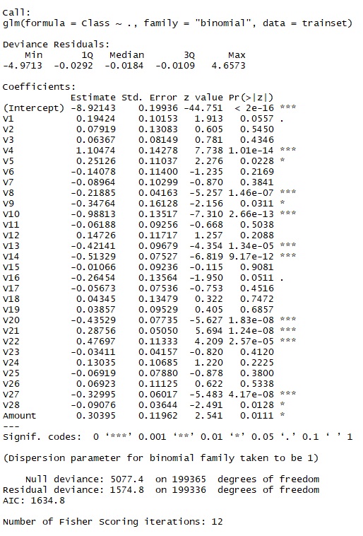
The coefficients table gives the estimate values for the coefficients, or the betas, for our logistic regression model.

Coefficients positive means that higher values in these two variables are indicative of fraud. Star means the variables are significant in our model.

To evaluate the performance of a logistic regression model, the following metrics are considered:

• AIC (Akaike Information Criteria). AIC (Akaike Information Criteria) is a measure of the quality of the model. A low AIC is desirable.
• Null Deviance. Null deviance shows how well the response is predicted by a model with nothing but an intercept (grand mean)
• Residual Deviance

In addition, we run the anova() function on the model to analyze the table of deviance.

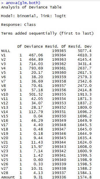
GLM Prediction

We assess the predictive ability of the model on the test dataset and then we convert the glm output probabilities to predictions using a threshold value of 0.5. We aim to optimize the threshold to minimize the False Negative Rate by increasing the classification threshold with the risk of identifying some legitimate transactions as fraudulent.

GLM Evaluation

From the metrics computation, we have the following prediction performance metrics for the logistic regression

Metrics	GLM performance
AUC	0.969
AUPRC	0.771
Accuracy	0.999
Precision	0.879
Recall	0.646
F1	0.745

Decision trees

classification and regression tree (CART) approach was developed by Breiman et al. (1984). Decision tree builds classification or regression models in the form of a tree structure. Here, we predict a categorical variable so we build a classification tree. The recursive partitioning algorithm creates a set of rules, splitting the data set into smaller and smaller subsets to incrementally develop the final result: a classification tree with decision nodes and leaf nodes.

DT implementation

In R, CART (Classification & Regression Trees) is done with R, Rpart .When it comes to pre-processing, tree-based methods performs usually well on unprocessed data (without normalizing, centering, scaling features).

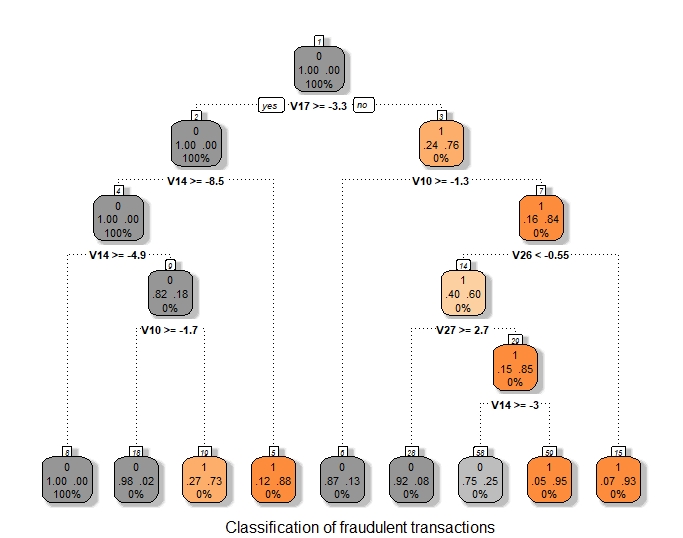
DT visualization

The decision rules generated by the CART (Classification & Regression Trees) predictive model is visualized as a binary tree. The leaves are the classification we assign to the target Class.

DT Prediction

Following the prediction, we visualize the confusion matrix.

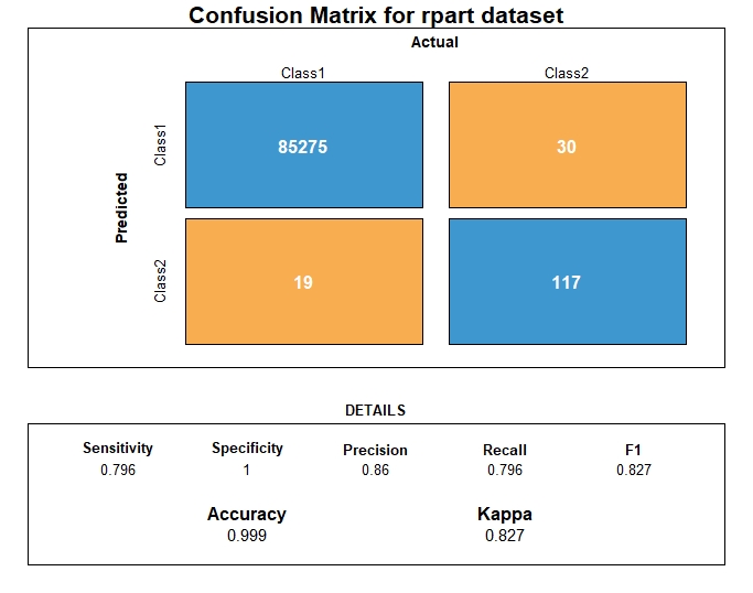
DT Evaluation

From the metrics computation, we have the following prediction performance metrics for the decision tree algorithm.

Metrics	DT performance
AUC	0.897
AUPRC	0.686
Accuracy	0.999
Precision	0.860
Recall	0.795
F1	0.826

Ensemble - Bagging

What is Bagging?

Bootstrap aggregating (bagging) aims to decrease the model’s variance with parallel ensemble methods where the base learners are generated in parallel and trained by the same algorithm to individually predict the outcome. The final prediction is then decided by the majority of the votes as the ensemble simply averages the predicted values. In this project, Bagging was implemented through Random Forest.

Bagging with Random forest

Random Forest is an Ensemble classifier which uses first multiple decision trees as weak learners to, then, bootstrap aggregate, a process called “bagging”, the tree learners. Random Forest output is a stronger classifier.

Note the main difference between Random Forests and XGBoost: in Random Forests, trees are independent, and as, in boosting, the tree N+1 focus its learning on the loss (what has not been modeled by the tree N).

RF Implementation

The module used is R, RandomForest based on Breiman and Cutler’s Random Forests for Classification and Regression.

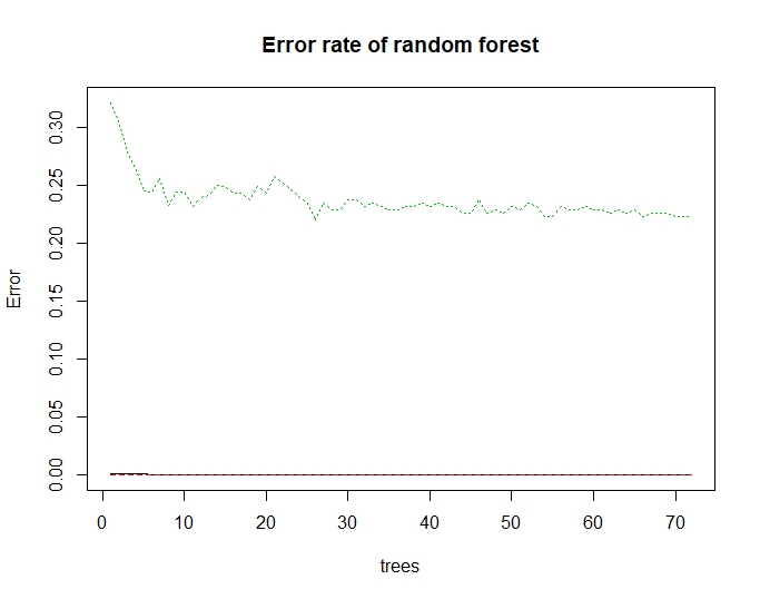
RF Hyperparameters setting

To build our model, we first need to set the number of trees. This number is the lower which minimizes the error.

RF model building

To optimize the parameters, we plot the Error vs Number of trees Graph.

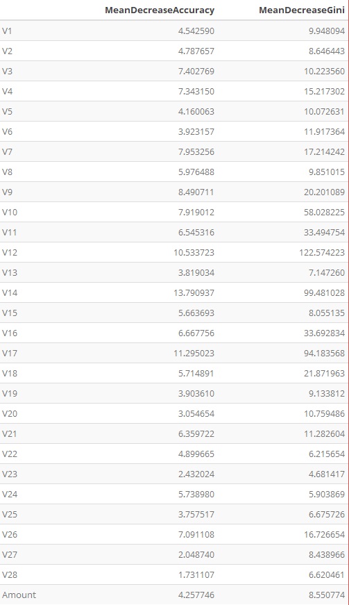
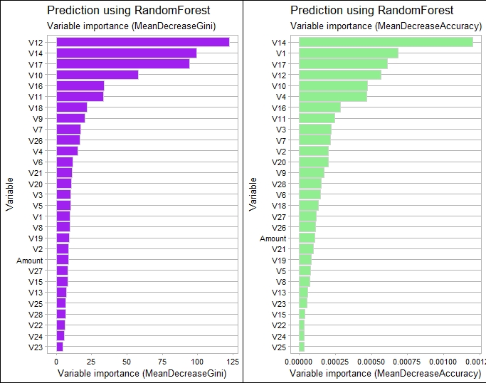
RF Features importance

Random Forest makes it possible to measure the relative importance of each feature on the prediction. We look particularly at:

• Gini Importance or Mean Decrease in Impurity
• Permutation Importance or Mean Decrease in Accuracy

RF Prediction

Following the prediction on the test dataset, we visualize the confusion matrix and related metrics.

RF Evaluation

From the metrics computation, we have the following prediction performance metrics for Random Forest

Metrics	RF performance
AUC	0.901
AUPRC	0.747
Accuracy	0.999
Precision	0.929
Recall	0.802
F1	0.861

Ensemble - Boosting

Boosting

Boosting goal is to decrease the model’s bias with sequential ensemble methods where the base learners are generated sequentially sequential ensemble. By combining the outputs of many “weak” classifiers to produce, at each iteration, from the whole ensemble learnt so far, a powerful final “ensemble”. In this project, Boosting models were Adaboost, Xgboost, Gradient Boosting Machine.

AdaBoost

AdaBoost, short for Adaptive Boosting, is a legacy machine learning ensemble algorithm formulated by Yoav Freund and Robert Schapire in 1996. In 2000, Friedman et al. developed a statistical view of the AdaBoost algorithm as stage wise estimation procedures for fitting an additive logistic regression model, minimizing its exponential loss function. The weak learners in AdaBoost are decision trees with a single split, called decision stumps. Once the classifiers have been trained, they can be used to predict new data.

Implementation

In this project, I have used the r, fastAdaboost package In term of data preparation, AdaBoost is sensitive to noisy data and outliers.

Hyperparameters setting

The number of iteration has been set up at 5

Prediction

Predictions are made by calculating the weighted average of the weak classifiers. The prediction for the ensemble model is taken as a sum of the weighted predictions. If the sum is positive, then the first class is predicted, if negative the second class is predicted.

Evaluation

From the metrics computation, we have the following prediction performance metrics for Adaboost

Metrics	AdaBoost performance
AUC	0.955
AUPRC	0.848
Accuracy	0.999
Precision	0.795
Recall	0.914
F1	0.850

XGBoost

XGBoost relies on Gradient Boosting, a machine learning technique for regression and classification problems, which produces a prediction model in the form of an ensemble of weak prediction models, typically decision trees. It builds the model in a stage-wise fashion like other boosting methods do, and it generalizes them by allowing optimization of an arbitrary differentiable loss function. XGBoost is one of the implementations of Gradient Boosting concept, but what makes XGBoost unique is that it uses “a more regularized model formalization to control over-fitting, which gives it better performance,” according to the author of the algorithm, Tianqi Chen. XGBoost performance optimization is achieved through parallelization of tree construction, distributed or out of core Computing, and cache optimization.

Implementation

To implement XGBoost, R, XGboost package is used. XGBoost requires the predictors to be numeric and to have both training and test data in numeric matrix format.

Hyperparameters setting

The hyperparameters to be set are:

• max Number of Iterations - nrounds = 100
• gamma = 0.1
• max_depth = 10
• objective = “binary:logistic”

Building the model

Each line shows how well the model explains our data. Overfitting after a number of iteration means the number of rounds should be reduced.

Feature Importance

Each feature is grouped by importance with k-means clustering. We build the feature importance data table as XGBoost shows which predictors are the most influential on the Classification prediction.

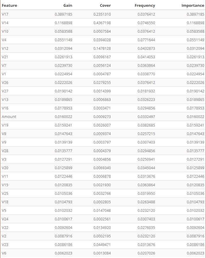
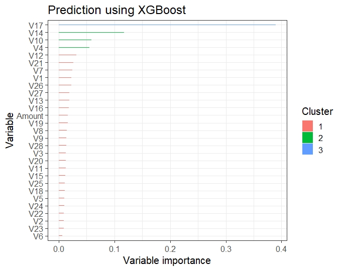
• Features Importance table
• Gain is the improvement in accuracy that the addition of a feature brings
• Plotting the feature importance

Prediction

We then test the model by applying it to the test data and we visualize the prediction results using the confusion matrix.

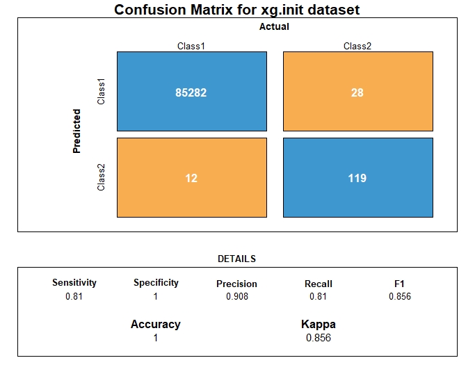
Evaluation

From the metrics computation, we have the following prediction performance metrics for XGboost

Metrics	XGBoost performance
AUC	0.979
AUPRC	0.891
Accuracy	0.999
Precision	0.908
Recall	0.809
F1	0.856

Model evaluation and selection

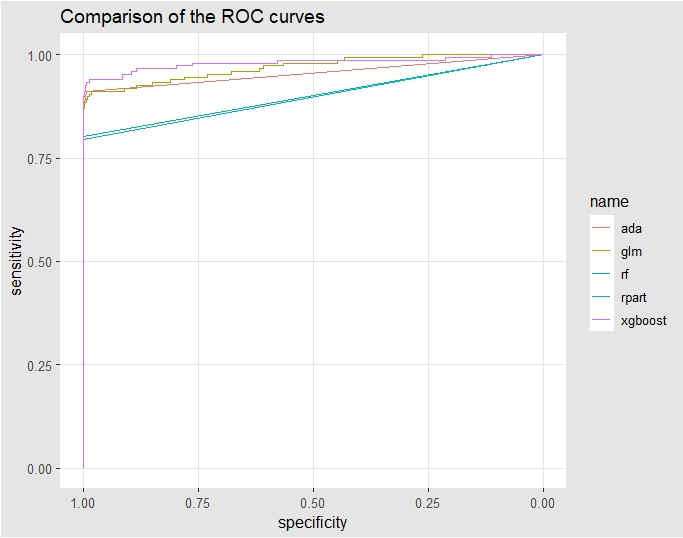
To compare prediction performance between the different models, we will use: ROC AUC, Recall, Precision, F1 and Matthews Coefficient

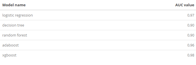
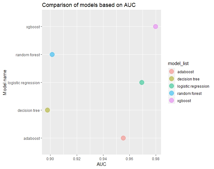
ROC AUC comparison

Comparing the different re-sampling techniques based on AUC, AUC is higher in decreasing order for

1. XGBoost
2. Logistic regression
3. AdaBoost

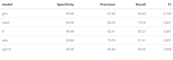
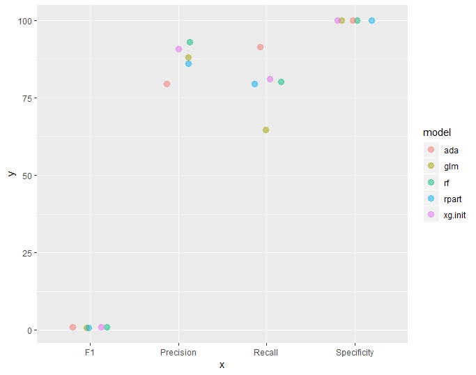
Recall, Precision, F1 comparison

In the table and plot below, the following metrics were grouped and then plotted.

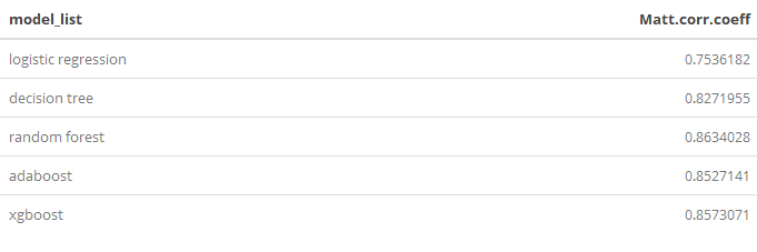
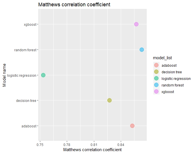
Matthews Coefficient comparison

For each model, the Matthews correlation coefficient were computed and compared.

Results and findings

At this stage, we evaluate the final model on the test hold-out data and when assessing the final results, we meet our objective, to be able to achieve relatively good predictions so to prevent fraud.